Some quick stats from the PSRC Parcel-based model

Exported using the opus_data_to_sql tool from the seattle_parcel example project.

Let the data drive the simulation...what's unclear without digging through the logs is how much of this is synthetic or allocated by disaggregating larger areas, or alternately, how much is a real parcel/building/job. Of course it's been stated (several times in the user guide) it's just an example.

300 pages and still not seeing the one important one (if it exists) that explains a typical workflow of how to get important data into the above format...

I'm thinking of starting with the ABS publication:
3218.0 Population Estimates by Statistical Local Area, 2001 to 2009
http://www.abs.gov.au/AUSSTATS/abs@.nsf/DetailsPage/3218.02008-09?OpenDocument

Since it contains 63 Statistical Local Areas within Sydney, it seems like a reasonable starting point for a zone-based model, i.e. not departing from the above too much in general terms of zones (factor of 1/4 the number of zones, and 9 times the population).

Starting to look like refactoring/modelling = easy, useful data = very hard.

When You Put Data In, You Are Able to Get It Out

A valuable part of any software solution is the ability to export your data. I've already covered a bit about more detailed analysis of data within OPUS, however OPUS also comes with a decent array of import and export tools.

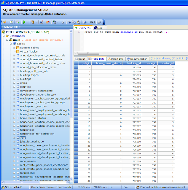
As an example of how I go about finding and using these, here's a quick export to SQLite3:

1. Open OPUS 4.3.1 (or later).
2. File > Open Project > san_antonio_zone.xml
3. On the Data Tab, select the Tools Tab, navigate down to the tool_library
4. Find opus_data_import_export_tools > opus_data_to_sql_tool
5. Right-click and choose the first option - Execute Tool...
   
   
   
6. Configure the variables as required.
7. Click Execute Tool

 

• As I just wanted to get in there without the overhead of dealing with MySQL, PostGreSQL, MS SQL or another DBMS and performance is not a hugely significant issue, I rolled with the preconfigured sqlite_test_database_server. (To add more, you can configure these in the top menu bar > Tools > Database Connections dialog)
• For SQLite3, the database name is just the file location. At least on Windows 7 x64, it appends ".txt" to the file name (even though I asked for a ".db3" file for reasons I'll explain shortly).
• The opus_data_directory is either:
• C:\opus\data\san_antonio_zone\base_year_data
• C:\opus\data\san_antonio_zone\runs\run_2.run_2011_01_21_13_35 (replaced with the relevant run)
• Year is self-explanatory. Don't include it in the opus_data_directory path above.

Why .db3? It's associated with SQLite 2009 Pro Enterprise Manager / SQLite3 Management Studio. (shortcut to download) (other tools here)
This makes exploring the raw data far easier because you don't have the external dependency on a DBMS.

Aside: Probably one of the reasons SQLite3 is bundled with recent versions of Python, and dominates the embedded/mobile data storage space.

For example, let's explore and compare 2006 to 2005 in the example San Antonio:

• In 2006, the simulation determined households increased to 546,786 rows, up 2.5% from 533,331 rows in the base_year_data (2005).
• Also in 2006, the simulation determined jobs increased to 762,339 rows, up 7.3% from 710,325 rows in 2005.

2005 Base Year Data has many more estimation variables, constraints, control totals, model coefficients and other configuration variables

2006 Simulated Data has significantly fewer - it should only be storing computed or modified data

And (click for larger version), we can start seeing precisely how the sample model's designers chose to implement their various components. For example, I can see that a zone is just a table containing the columns zone_id, schl_district, dev_acre, totacres, travel_time_to_airport, rd_density and travel_time_to_cbd.

There also appears to be no change from 2005 to 2006 in these rows, though without exporting and comparing the entire individual tables I couldn't say calculations weren't being performed on this dataset.

The key message ultimately is - OPUS is a platform upon which you can build in whatever model semantics you desire.

It isn't some blind experiment you enter data into hoping you have a working city coming out the other side, it's a collection of existing real-world (or synthesised) data, and a list of models grouped together into scenarios representing possible futures - futures based on anything from our best judgement, to our knowledge of current and historical events, to our wildest fantasies.

What story do you want to tell today? How probable do you think it is? How well supported by the data is it?

Understanding the OPUS User Guide

Sometimes it's hard while learning to know what's really significant or important. Like reading big chunks of a 300 page manual in depth, I think I'd find it hard to make a compelling case for things like how the MNL (multinomial logit) model is an efficient discrete choice model for doing things like modelling economic utility (assuming I'm not mincing terms together).


But let's not let that detract from some useful or interesting pieces (at least for me) which really have helped to establish some meaningful context.

For a start, let's read into how the manual is structured. The 6 graph nodes represent chapters in order in the OPUS manual. I've added some comments from my understanding so far of the actual implementation's useful features:

 

Let's consider some other diagrams in the OPUS User Guide. 

OPUS User Guide v4.3, Page 32, Chapter 7.1, Figure 7.2: Opus databases, datasets and arrays

A good clarification of concepts, including in the surrounding text that these .li4 files are just numpy arrays. As implied earlier, we'd get data into this format by using the import tools on the Data->Tools tab.

OPUS User Guide v4.3, Page 96, Chapter 17.2.1, Figure 17.3: Overview of UrbanSim Model System

Note: A similar if not equivalent diagram (with a different visual style) appears as Figure 2.1: UrbanSim Model Components and Data Flow on page 15.

This overview is explained to be the general template many urban planners use to calibrate their instance of UrbanSim. We can easily see the important and required inputs and other likely dependencies for which data will need to be identified (or synthesised / worked around) in order to get a new city into OPUS, and which models such data is relevant to.

OPUS User Guide v4.3, Page 54, Chapter 10.2.1, Figure 10.2: Using the "Result Browser" for interactive result exploration

And then there's the that's (hopefully) just plain cool diagrams!

On a positive note

What's the interesting output an average person may actually be able to understand that comes out of OPUS? 

Things like animated GIFs, this one showing the years 2005-2019 of the zone_ln_emp_10_min OPUS indicator in the San Antonio zone model.

There isn't a great deal of change, but since the scale does increase over the years, you can see some of the zones changing to a different green.

Of course that's a pretty terrible story, but it demonstrates that the Mapnik dependency appears to be working correctly to generate visual output on Windows 7 x64, which means much more interesting stories should be able to be successfully told in future, with any luck about how machine learning methods compare to the classical economic modelling of cities.

(Yes I know the image is wider than Blogger's column, but since Blogger's thumbnails aren't animated and CSS doesn't allow quick scaling of images as far as I know - it would be something like img { height:75%; width: 75%; } if allowed ... and this is just a demo...it will do)

Modelling is ... easy?

Like the vast majority of software, there's the well travelled superhighway you can drive down rip-roaringly fast (or faster), and there's the jungle you're lucky if you get a machete to hack through the undergrowth with.

UrbanSim's proverbial superhighway is the existing types of models. If you can explain the difference between an Allocation Model and a Location Choice Model, you'll enjoy being able to quickly configure such models in the OPUS GUI (or worst case, modifying the underlying XML file).

If like me, you're still learning that difference, the best places to start seem to be:

1. The OPUS Users Guide and Reference for v4.3, Chapter 14 - Model Types in OPUS. A good amount of detail on the basic theory (though not the implementation) of Simple, Sampling, Allocation, Regression and Choice models.
2. The OPUS walkthrough tutorials on Creating New Models
1. Creating an Allocation Model
2. Creating a Regression Model

Of course if these models are insufficient for your needs, you'll be like me, looking for the machete (or hopefully bulldozer) to get through the jungle. At least for me, I'm coming back to the same core, it's not the syntax, it's the semantics. But the syntax helps in establishing context from which you learn to improve your understanding of semantics.... or something like that. It can be frustrating, which is probably a good thing.

/rant on

It can be an indicator that things like compiling your own code from source are in many cases too complex for even many IT professionals to deal with. And who has the time anyway?

On another note, UI has evolved. When you realise how the vast majority of iOS (which now has been force bundled with XCode for a 3.5GB download just to get XCode 3.2.5), Mac, PC, Android, Windows Phone 7, and web applications expose all text or actions to the user as big shiny buttons. My pet peeve so far is OPUS needs so much right-clicking on models, scenarios, indicators (and probably much more)....that important contextual information is not in the GUI exposed to the user, but hidden in menus the user must explicitly ask for.

Add to that learning a Mac...far harder than I expected, especially with the Python 2.6 + SIP + Qt + PyQt4 dependencies taking ages to compile and running into what I strongly suspect is a 32/64-bit compilation issue (of course code for any individual application must be compiled for one or the other, often explicitly) due to [paraphrased]

PyQt4.QtCore

ImportError: ...no suitable image found, did find ../QtCore.so: mach-o, but wrong architecture

/rant off

As one of my professors once said it's:

"where the rubber hits the road".

I suspect the best thing for me to do is probably try finding ways to be more participatory in the OPUS community, i.e. forums and whatever else is on www.urbansim.org

For now, back to coding/testing/debugging fun =)