When You Put Data In, You Are Able to Get It Out

A valuable part of any software solution is the ability to export your data. I've already covered a bit about more detailed analysis of data within OPUS, however OPUS also comes with a decent array of import and export tools.

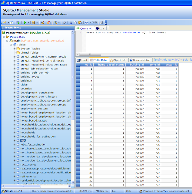
As an example of how I go about finding and using these, here's a quick export to SQLite3:

1. Open OPUS 4.3.1 (or later).
2. File > Open Project > san_antonio_zone.xml
3. On the Data Tab, select the Tools Tab, navigate down to the tool_library
4. Find opus_data_import_export_tools > opus_data_to_sql_tool
5. Right-click and choose the first option - Execute Tool...
   
   
   
6. Configure the variables as required.
7. Click Execute Tool

 

• As I just wanted to get in there without the overhead of dealing with MySQL, PostGreSQL, MS SQL or another DBMS and performance is not a hugely significant issue, I rolled with the preconfigured sqlite_test_database_server. (To add more, you can configure these in the top menu bar > Tools > Database Connections dialog)
• For SQLite3, the database name is just the file location. At least on Windows 7 x64, it appends ".txt" to the file name (even though I asked for a ".db3" file for reasons I'll explain shortly).
• The opus_data_directory is either:
• C:\opus\data\san_antonio_zone\base_year_data
• C:\opus\data\san_antonio_zone\runs\run_2.run_2011_01_21_13_35 (replaced with the relevant run)
• Year is self-explanatory. Don't include it in the opus_data_directory path above.

Why .db3? It's associated with SQLite 2009 Pro Enterprise Manager / SQLite3 Management Studio. (shortcut to download) (other tools here)
This makes exploring the raw data far easier because you don't have the external dependency on a DBMS.

Aside: Probably one of the reasons SQLite3 is bundled with recent versions of Python, and dominates the embedded/mobile data storage space.

For example, let's explore and compare 2006 to 2005 in the example San Antonio:

• In 2006, the simulation determined households increased to 546,786 rows, up 2.5% from 533,331 rows in the base_year_data (2005).
• Also in 2006, the simulation determined jobs increased to 762,339 rows, up 7.3% from 710,325 rows in 2005.

2005 Base Year Data has many more estimation variables, constraints, control totals, model coefficients and other configuration variables

2006 Simulated Data has significantly fewer - it should only be storing computed or modified data

And (click for larger version), we can start seeing precisely how the sample model's designers chose to implement their various components. For example, I can see that a zone is just a table containing the columns zone_id, schl_district, dev_acre, totacres, travel_time_to_airport, rd_density and travel_time_to_cbd.

There also appears to be no change from 2005 to 2006 in these rows, though without exporting and comparing the entire individual tables I couldn't say calculations weren't being performed on this dataset.

The key message ultimately is - OPUS is a platform upon which you can build in whatever model semantics you desire.

It isn't some blind experiment you enter data into hoping you have a working city coming out the other side, it's a collection of existing real-world (or synthesised) data, and a list of models grouped together into scenarios representing possible futures - futures based on anything from our best judgement, to our knowledge of current and historical events, to our wildest fantasies.

What story do you want to tell today? How probable do you think it is? How well supported by the data is it?